AR, MA, ARMA, ARMAX

데이터분석/분석-지도학습

AR, MA, ARMA, ARMAX

씩씩한 IT블로그 2020. 12. 28. 18:07

시계열 회귀분석의 종류인 AR, MA, ARMA 분석에 대해서 알아보고 실습을 진행해 본다.

1. AR, MA

(1) AR(p) model

Y_t가 Y_t의 p기 이전까지의 값에 의해 설명되는 모델

(2) MA(q) model

Y_t가 현재영향(e_t)으로 부터 과거 q기 전까지 영향(e_t-q)에 의해 설명되는 모델

2. ARMA

AR(p)와 MA(q)의 선형조합.

3. 파라미터 p,q는 어떻게 찾는가?

AR과 MA를 이용하여 분석을 수행하기 위해서는 파라미터 p,q값을 분석자가 결정해야 한다.

이 파라미터를 찾는 방법은 ACF와 PACF를 사용한다.

AR의 경우 PACF그래프에서 수렴하기 직전 마지막값이 p가 되고, MA의 경우 ACF그래프에서 수렴하기 직전값이 q가 된다.

이를 아래의 예시를 통해 보면

ACF그래프에서 1이 수렴하기 직전의 값이므로 MA의 모수 q=1이되고,

PACF그래프에서 1이 수렴하기 직전의 값이므로 AR의 모수 p=1이 된다.

* 그런데 실제로 분석을 해보면 항상 위와같이 수렴직전의 값이 p,q가 되진 않을때도 있다.

4. 최적모수를 찾은 후 ARMA분석

import warnings
warnings.filterwarnings('always')
warnings.filterwarnings('ignore')

import pandas as pd
import numpy as np
import matplotlib.pyplot as plt
import statsmodels.api as sm

# 데이터로딩 및 확인
data = sm.datasets.get_rdataset("deaths", "MASS")
raw = data.data
raw.value = np.log(raw.value) #정상화를 위해 로그화
raw.plot(x='time', y='value')
plt.show()

# ACF/PACF 확인
plt.figure(figsize=(10, 8))
sm.graphics.tsa.plot_acf(raw.value.values, lags=50, ax=plt.subplot(211))
plt.xlim(-1, 51)
plt.ylim(-1.1, 1.1)
plt.title("ACF")

sm.graphics.tsa.plot_pacf(raw.value.values, lags=50, ax=plt.subplot(212))
plt.xlim(-1, 51)
plt.ylim(-1.1, 1.1)
plt.title("PACF")
plt.tight_layout()
plt.show()

from itertools import product

# ARMA(p,q) 모델링
result = []
for p, q in product(range(4), range(2)):
    if (p == 0 & q == 0):
        continue
    model = sm.tsa.ARMA(raw.value, (p, q)).fit()
    try:
        result.append({"p": p, "q": q, "LLF": model.llf, "AIC": model.aic, "BIC": model.bic})
    except:
        pass
   
# 모형 최적모수 선택
result = pd.DataFrame(result)
display(result)
opt_ar = result.iloc[np.argmin(result['AIC']), 0]
opt_ma = result.iloc[np.argmin(result['AIC']), 1]

# ARMA 모델링(가장좋은모수를 넣었을때)
fit = sm.tsa.ARMA(raw.value, (opt_ar,opt_ma)).fit()
display(fit.summary())

5. ARMAX

ARMA모델에 X값을 추가한 모델.

예를 들어 아래와 같은 시간에 따른 두가지 feature가 있고 최종적으로 consump을 예측하고자 할때, m2도 독립변수로서 사용하는 모델.

import requests
from io import BytesIO
import pandas as pd
import numpy as np
import matplotlib.pyplot as plt
import statsmodels.api as sm

# 데이터 로딩 및 확인
source_url = requests.get('http://www.stata-press.com/data/r12/friedman2.dta').content
raw = pd.read_stata(BytesIO(source_url))
raw.index = raw.time
raw_using = raw.loc['1960':'1981',["consump", "m2"]]
raw_using.plot()
plt.show()

# 모델링
## --------------------------- ARMAX ---------------------------
fit = sm.tsa.ARMA(raw_using.consump, (1,1), exog=raw_using.m2).fit() 
display(fit.summary())

## 잔차 확인
fit.resid.plot()
plt.show()

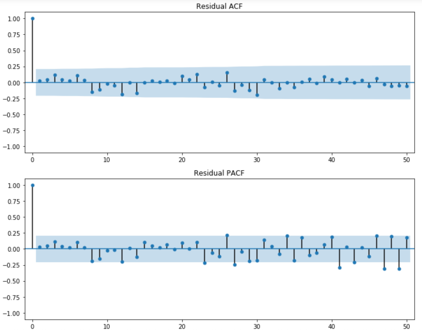
## 잔차 ACF/PACF
plt.figure(figsize=(10, 8))
sm.graphics.tsa.plot_acf(fit.resid, lags=50, ax=plt.subplot(211))
plt.xlim(-1, 51)
plt.ylim(-1.1, 1.1)
plt.title("Residual ACF")

sm.graphics.tsa.plot_pacf(fit.resid, lags=50, ax=plt.subplot(212))
plt.xlim(-1, 51)
plt.ylim(-1.1, 1.1)
plt.title("Residual PACF")
plt.tight_layout()
plt.show()