통계 자료 요약

# [백분위수 구하기]
from statistics import variance, stdev
import numpy as np

coffee = np.array([202,177,121,148,89,121,137,158])

#백분위수
cf_quant_20 = np.percentile(coffee, 20)
cf_quant_80 = np.percentile(coffee, 80)
print("20 Quantiles : ", cf_quant_20 )
print("80 Quantiles : ", cf_quant_80 )

#IQR 
q75, q25 = np.percentile(coffee, [75, 25])
cf_IQR = q75-q25
print("Inter quartile range:",cf_IQR)

20 Quantiles :  121.0
80 Quantiles :  169.4
Inter quartile range: 41.75

 

# [변동계수]
# 표준편차/평균

from statistics import variance, stdev
import numpy as np

coffee = np.array([202,177,121,148,89,121,137,158])

#CV
cf_cv = stdev(coffee)/np.mean(coffee)
cf_cv = round(cf_cv,2)
print("CV:", cf_cv)

CV: 0.25

 

# [도수 분포표]
import numpy as np
import pandas as pd

# 주량 데이터
drink_cup = pd.DataFrame({'cup' :[22,7,19,3,10,8,19,7,15,9,35,5],'who' : [ 'A', 'E', 'D', 'B', 'C','A','A','A','D','B', 'C','B']})


# 도수분포표
factor_cup = pd.cut(drink_cup.cup, 4) #네그룹으로 나누기
group_cup = drink_cup['cup'].groupby(factor_cup) #factor_cup 기준으로 묶기
count_cup = group_cup.agg(['count']) 

print(count_cup)

               count
cup                 
(2.968, 11.0]      7
(11.0, 19.0]       3
(19.0, 27.0]       1
(27.0, 35.0]       1

 

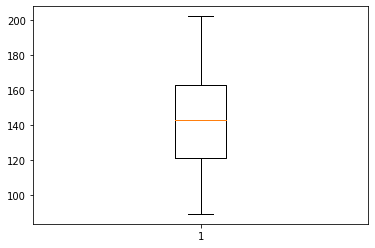
# [boxplot]

import numpy as np
import matplotlib.pyplot as plt

#카페인 함유량
coffee = np.array([202,177,121,148,89,121,137,158])

#상자그림
fig, ax = plt.subplots()
## 여기에 코드를 작성해주세요

plt.boxplot(coffee)
##
plt.show()

 

# [산점도 그리기]

import matplotlib.pyplot as plt
import pandas as pd
# body.csv 읽어오기 
body = pd.read_csv("body.csv")

# Q1. 산점도 
##1-1 키와 몸무게간 산점도 
fig, ax = plt.subplots()
plt.scatter(body['height'], body['weight'])
plt.show()
fig.savefig("height_weight_plot.png")

##1-2 키와 체지방량 산점도 
fig, ax = plt.subplots()
plt.scatter(body['height'], body['body_fat'])
plt.show()
fig.savefig("height_fat_plot.png")


##1-3 키와 다리길이 산점도 
fig, ax = plt.subplots()
plt.scatter(body['height'], body['leglen'])
plt.show()
fig.savefig("height_leglen_plot.png")



##1-4 키와 모발 산점도 
fig, ax = plt.subplots()
plt.scatter(body['height'], body['hair'])
plt.show()
fig.savefig("height_hair_plot.png")

 

키와 몸무게

 

# [공분산]
from statistics import variance, stdev
import numpy as np 
import pandas as pd

# body.csv 읽어오기 
body = pd.read_csv("body.csv")

# 공분산
cov_body = cov_body = body.cov()

print(cov_body)

                 height     weight  muscle_mass   body_fat     leglen  \
height       142.050000  44.607316    11.784461  32.980749  92.332500   
weight        44.607316  39.346241     8.641430  34.839548  28.994755   
muscle_mass   11.784461   8.641430    39.819721 -31.334680   7.659900   
body_fat      32.980749  34.839548   -31.334680  76.991671  21.437487   
leglen        92.332500  28.994755     7.659900  21.437487  60.016125   
hair          -1.420500  -0.446073    -0.117845  -0.329807  -0.923325   

                 hair  
height      -1.420500  
weight      -0.446073  
muscle_mass -0.117845  
body_fat    -0.329807  
leglen      -0.923325  
hair         0.014205  

 

 

# [상관계수]
from statistics import variance, stdev
import numpy as np 
import pandas as pd

# body.csv 읽어오기 
body = pd.read_csv("body.csv")

# 공분산
cov_body = cov_body = body.cov()

print(cov_body)

                 height     weight  muscle_mass   body_fat     leglen  \
height       142.050000  44.607316    11.784461  32.980749  92.332500   
weight        44.607316  39.346241     8.641430  34.839548  28.994755   
muscle_mass   11.784461   8.641430    39.819721 -31.334680   7.659900   
body_fat      32.980749  34.839548   -31.334680  76.991671  21.437487   
leglen        92.332500  28.994755     7.659900  21.437487  60.016125   
hair          -1.420500  -0.446073    -0.117845  -0.329807  -0.923325   

                 hair  
height      -1.420500  
weight      -0.446073  
muscle_mass -0.117845  
body_fat    -0.329807  
leglen      -0.923325  
hair         0.014205