[RNN] LSTM으로 감성분석

1. tensorflow keras

import tensorflow as tf
from tensorflow.keras import layers
from tensorflow.keras.datasets import imdb
from tensorflow.keras.preprocessing import sequence

 

2. 최대 단어 개수와 길이

# 최대 단어의 개수
max_features = 10000 
# 최대 단어 길이 (한번의 인풋당 들어갈 단어의 수)
maxlen = 200   

# num_word : 빈도가 높은 상위 max_features개 단어만 사용함.
# skip_top : 빈도가 높은 상위 단어 0개 제외
(input_train, y_train), (input_test, y_test) = imdb.load_data(num_words=max_features, skip_top=0)

 

3. 전처리

# sequence.pad_sequences : maxlen보다 작으면 앞을 0으로 채우고, maxlen보다 크면 앞을 자른다.
X_train = sequence.pad_sequences(input_train, maxlen=maxlen)
X_test = sequence.pad_sequences(input_test, maxlen=maxlen)


'''
input_train과 input_test는 모두 2차원 데이터. 각행의 길이는 모두 다르다. 
X_train은 pad를 통해 각행의 길이가 모두같다(maxlen로)

'''
print(X_train.shape)
print(X_test.shape)

# 2차원에서도 모든요소 값 중 max값을 반환한다 (= 9999이므로 0~9999->10000개)
print(X_train.max())

<<output>>
(25000, 200)
(25000, 200)
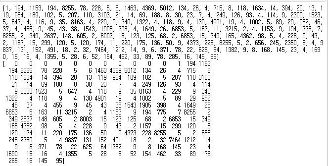
9999

print(input_train[1])
print(X_train[1])

 

4. 계층적 모델 구성

model = tf.keras.Sequential()
model.add(layers.Embedding(max_features,32))
model.add(layers.LSTM(32))
model.add(layers.Dense(1, activation='sigmoid'))

model.compile(optimizer='rmsprop', loss='binary_crossentropy', metrics=['acc'])
hist = model.fit(X_train, y_train, 
                   epochs=10,
                   batch_size=128,
                   callbacks=[tf.keras.callbacks.EarlyStopping(monitor='val_loss', patience=3)],
                   validation_split=0.2)

 

5. 파라미터 확인

'''
[파라미터계산]

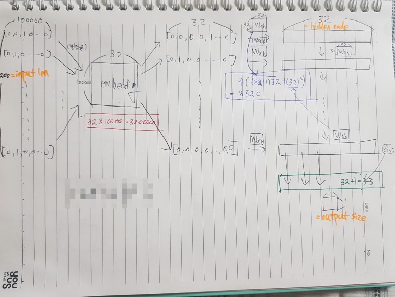
1. embedding_1 : 
10000개의 단어를 32개로 분류하는 작업. len가 10000로 원핫코딩된([0,0,0,0,...1,0,...0]) 한가지 단어를 32개로 대표되는 
단어들 중 하나로 분류하는 작업. 즉 하나의 len==10000인 인풋이 들어오면 10000*32 행렬을 통해 len==32인 하나의 아웃풋 
([0,0,0,0,...1,0,0,0])으로 만들어 주는 역할. 
<cal : 10000 * 32 = 320000 >

2. lstm_1 : 
W_xh, W_hh를 계산. 4((인풋의크기+1)*아웃풋의크기 + 아웃풋의크기^2) = 4((c+1)*h+h^2)
W_xh : (c+1)*h
W_hh : h^2
4 neural networ layer {W_forget, W_input, W_output, W_cell} : *4
<cal : 4((32+1)*32+32^2=8320>

3. dense_1:
<cal : (32+1)*1=33>

'''

model.summary()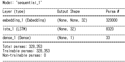

 

6. 시각화

import matplotlib.pyplot as plt

fig, loss_ax = plt.subplots(figsize=(8, 5))

acc_ax = loss_ax.twinx()

loss_ax.plot(hist.history['loss'], 'y', label='train loss')
loss_ax.plot(hist.history['val_loss'], 'r', label='val loss')

acc_ax.plot(hist.history['acc'], 'b', label='train acc')
acc_ax.plot(hist.history['val_acc'], 'g', label='val acc')

loss_ax.set_xlabel('epoch')
loss_ax.set_ylabel('loss')
acc_ax.set_ylabel('accuray')

loss_ax.legend(loc='upper left')
acc_ax.legend(loc='lower left')

plt.show()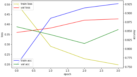

import matplotlib.pyplot as plt

acc = hist.history['acc']
val_acc = hist.history['val_acc']
loss = hist.history['loss']
val_loss = hist.history['val_loss']

epochs = range(len(acc))

plt.plot(epochs = range(len(acc)))

plt.plot(epochs, acc, 'bo', label='Training acc')
plt.plot(epochs, val_acc, 'b', label='Validation acc')
plt.title('Training and validation accuracy')
plt.legend()

plt.figure()

plt.plot(epochs, loss, 'bo', label='Training loss')
plt.plot(epochs, val_loss, 'b', label='Validaiton loss')
plt.title('Training and validation loss')
plt.legend()

plt.show()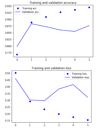

 

7. 모델 테스트

score = model.evaluate(X_test, y_test)
print('test_loss: ', score[0])
print('test_acc: ', score[1])

test_loss:  0.35294207727432253
test_acc:  0.86456